Lecture 1: Introduction

Geostatistics

J Mwaura

What is Geostatistics?

Set of models and tools used for statistical analysis of continuous data

Nature of data:

  1. Measured at a spatial location
  2. Number of sampled points are limited
  3. Constitutes of errors, as such predictions results should also have uncertainity information

Geostatistical analysis goal is to predict values where no data have been collected

Data Features

Exploring characteristics of data is the first step in data analysis

Helps to develop insights about the data

The features are:

  • Dependency
  • Stationarity
  • Distribution

Data Dependency

Independent data does not need geostatistical analysis - data isn't predictable

Thus, for geostatistical analysis use spatially dependent data

Tools to detect spatial dependence;

  • Exploratory Spatial Data Analysis (ESDA)
    • Helps to select optimum geostatistical modal e.g. lognormal, gausssian etc
  • Geostatistical Wizard

Methods offered by tools - covariogram, correlogram and variogram

Data Stationarity

Geostatistics uses stationary data

Non-stationary data needs conversion

Conversion methods

  1. Data detrending
  2. Data transformation

Data Distribution

Geostatistics works optimal when input data are Gaussian

If not, data have to be transformed to be close to Gaussian distribution

Transformation approaches:

  • Data normalization

Random Variables

This is a variable whose possible values are numerical outcomes of a random phenomenon

Types of random variables;

  • Discrete
  • Continuous

Modeling of discrete data calls for point pattern analysis

Random variables are variables that cannot be predicted with complete certainty. This calls for probability

Probability Distributions of Discrete Variables

Binomial Probability Distribution

Poisson Probability Distribution

Boltzmann Probability Distribution

Probability Distributions of Continuous Variables

Normal (Gaussian) Probability Distributions

Standard Normal Probability Distribution

Exponential Probability Distribution

Properties of Random Variables

  • Stationarity - location (central tendency). States as follows
    • Correlation between any 2 locations depends only on the vector that links them, not their exact locations
    • Mean of a variable at one location is equal to the mean at any other location
    • Data variance is constant in the area under investigation
  • Dispersion (variability)

Stationarity

Stationarity means that statistical properties do not depend on exact locations

Spatial correlation is modeling as a function of distance between pairs of locations

Spatial correlation functions;

  • Covariance
  • Semivariogram

Data Modeling - Kriging

Kriging assumes spatial autocorrelation or dependency- near things are more alike than those farther away

Krige models;

  1. Spatial dependency
  2. Semivariogram

Modeling outputs maps are; prediction, prediction standard errors, probability, and quantile

Kriging

Kriging uses covariance and semivariograms to optimaze predictions

It is a spatial interpolation method or optimum interpolator

Kriging prediction and prediction uncertainity depend on covariances or semivariograms

Semivariogram and Covariance

Steps to develop semivariogram

  • Find all pairs of measurements (any two locations)
  • Calculate for all pairs the squared difference between values
  • Group vectors (or lags) into similar distance and direction classes - referred as binning
  • Average the squared differences for each bin

Semivariogram and Covariance Estimation

Covariance estimation uses data mean, but data mean is usually unknown, but estimated, this causes errors

Thus, semivariogram is normally a preferred function tool to characterize spatial data structure

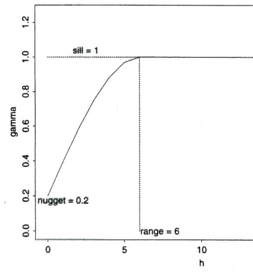
Variogram Parameters

Nugget

    Represents micro-scale variation or measurement errors

Sill

    Represents the variance of the random field

Range

    Distance at which data are no longer autocorrelated

ESDA Tools

Data distributions

Outliers - local and global

Trends - global

Spatial correlation and covariations

Interpolation Models

  1. Mechanical/Deterministic models
  2. Actual/empirical parameters are used and no estimate of the model error

    no strict assumptions about the variability of a feature exist. These models based on;

    • Distances between points e.g. Thiessen polygons, Inverse distance interpolation, Regression on coordinates, Natural neighbors, Splines
    • Degree of smoothing e.g. Radial Basis functions, local polynomials
  3. Linear statistical/Probability models
  4. Expert-based systems

Interpolation Models

  1. Linear statistical/Probability models
  2. Estimated parameters are used - estimation using probability theory

    An estimate of the prediction error available

    Data must satisfy strict statistical assumptions

    • kriging (plain geostatistics)
    • environmental correlation (e.g. regression-based)
    • Bayesian-based models (e.g. Bayesian Maximum Entropy)
    • hybrid models (e.g. regression-kriging)
    • geographically weighted regression (GWR)
  3. Expert-based systems

Interpolation Models

  1. Expert-based systems
  2. Data dependent models

    Predictions are different for each run

    Largely based on probability theory (especially Bayesian statistics). Examples;

    • knowledge-driven expert system (e.g. hand-drawn maps)
    • data-driven expert system (e.g. based on neural networks)
    • machine learning algorithms (purely data-driven)

Interpolators

Exact

Inexact of filtered

Exact Interpolators

measured and estimated values coincide

  1. IDW
  2. Radial basis functions
  3. Kriging

Inexact Interpolators

measured and estimated values do not have to coincide

  1. Global polynomials
  2. Local polynomials
  3. Kriging

Geographically Weighted Regression

The variograms and regression models are estimated locally - geographical space considered

Helps to study local differences in responses to input variables

The 2 main problems with GWR;

  1. Strong multicollinearity effects among coefficients make the results even totally wrong
  2. Loses degrees of freedom in the regression model

Validation of spatial prediction models

The true quality of a map can be best assessed by comparing estimated values with actual observations at validation points

  1. The mean prediction error (ME)
  2. The root mean square prediction error (RMSE)
  3. Cross-validation i.e. by subsetting the original point set in two data set - calibration and validation - and then repeating the analysis. Examples of cross-validation methods; k-fold, leave-one-out, Jackknifing

End of Lecture 1

Geostatistics

That's it!

Queries about this Lesson, please send them to: jmwaura.uni@gmail.com

References

  • Introduction to Modeling Spatial Processes using Geostatistical Analyst Konstantin Krivoruchko
  • The principles of geostatistical analysis Geostatistical Analyst
  • A Practical Guide to Geostatistical Mapping Tomislav Hengl
Courtesy of Open School
Geostatistics