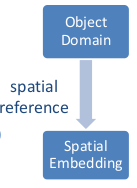
Spatial object/Geoobject: element to model real world data in geographic information system
Are described by spatial data (geodata)
Spatial information: custom-designed spatial data
The difference is?
- Geometry
- Topology
Spatial object/Geoobject: element to model real world data in geographic information system
Are described by spatial data (geodata)
Spatial information: custom-designed spatial data
The difference is?
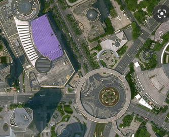
https://www.intelligence-airbusds.com/imagery/constellation/pleiades-neo/
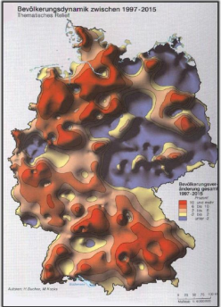
Exists everywhere, without boundaries
Complete
Collectable only on distinct points
Examples: ground level, temperature, precipitation, air pressure, accessibility
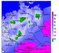
www.wetteronline.de
https://stackoverflow.com
Object-based
Field-based
Object-based
Field-based
Continuous
Differentiable
Isotropic - Independent of direction
Anisotropic - Properties vary with direction
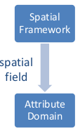
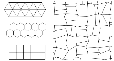
Spatial framework: a partition of a region of space
visualization tool: [Lu13]
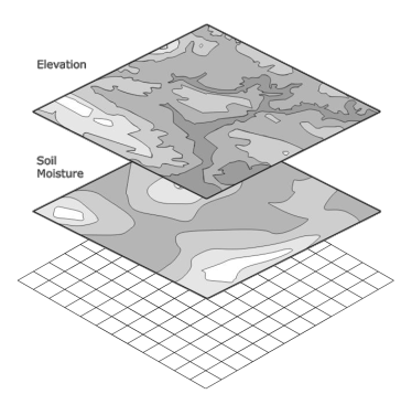
Layer
http://worboys.duckham.org/
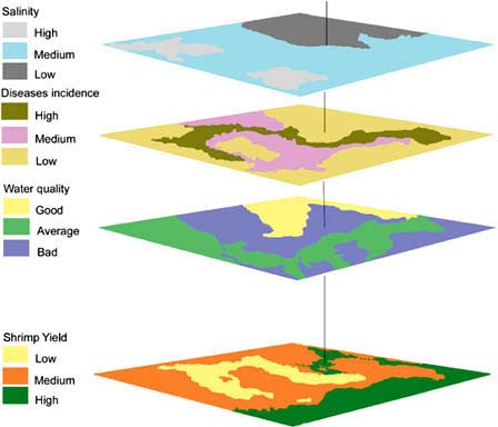
https://www.fao.org/3/y4816e/y4816e0g.htm
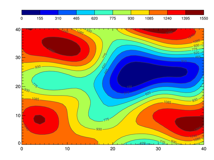
In the special case where - the spatial framework is a Euclidian plane and
The attribute domain is a subset of the set of real numbers then
A field may be represented as a surface in a natural way
Author: H.Bucher
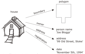
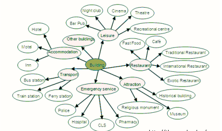
Object-based models decompose an information space into objects or entities
http://worboys.duckham.org/
Geometry
http://upload.wikimedia.org/
Topology
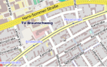
http://www.openstreetmap.de/
Topological transformations - Invertible, bijective, and continous (homeomorphism, elastic deformation)
• Translation • Rotation • Stretching • Reflection • Distortion
Topological properties (invariants):
The result of applying a topological transformation to a point-set is a topologically equivalent point-set
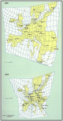
Authors: K.Splekermann, M.Wegener
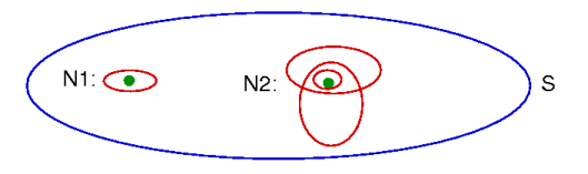
Focus on sets of points, the concepts of neighbourhood, nearness, and open set
All topological properties are definable in terms of the single concept of neighbourhood
A topological space is a collection of subsets of a given set of points S, called neighbourhoods, that satisfy the following conditions
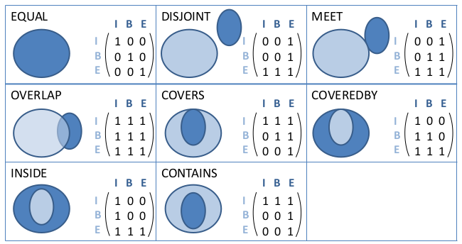
Formal description of binary topological relations: 9-intersection model
Intersections between interior, boundary and exterior of objects
512 possible, 8 reasonable matrices (for polygons)
Levels or scales of measurement
Level of measurement refers to the relationship among the values that are assigned to the attributes for a variable

Layer concept
Class concept
The entries of the matrix (numerical values representing the object identifier or attribute values) are interpreted as grey scale values
Euclidian distance is not defined
Points can only be represented by approximation
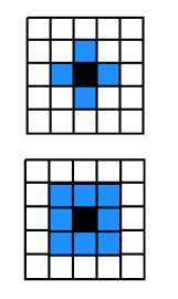
Basic morphological operations: • Dilatation • Erosion
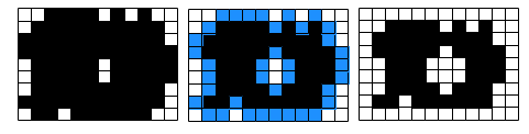
Particularly suited to describe continuous and areal themes
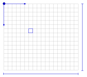
Refined raster: representation of objects is more accurate but also higher memory requirements and computing time
Guideline: raster width half as wide as the smallest element/distance which should be represented
Lossless compression techniques
Stores the direction in which pixels with the same value are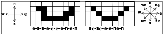
Stores the number of adjacent pixels with the same value in a row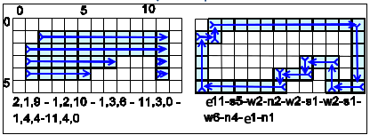
Lossless compression techniques
Decomposition into squares which are as big as possible. Only the position and size of the squares has to be stored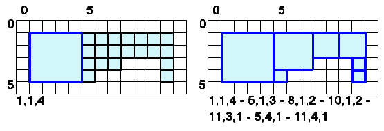
Three examples (Greedy approach)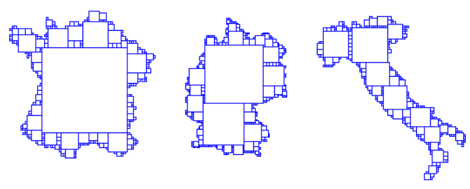
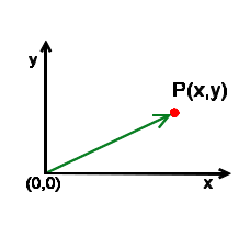
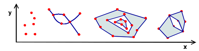
Requisite: two or three dimensional cartesian coordinate system with euclidian metric
Line based model (edge representation)
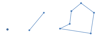
Basic element: point
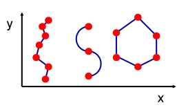
Line segment • Defined by two points
Line: adjacent line segments
Surface or polygon: closed line
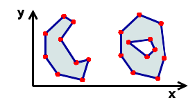
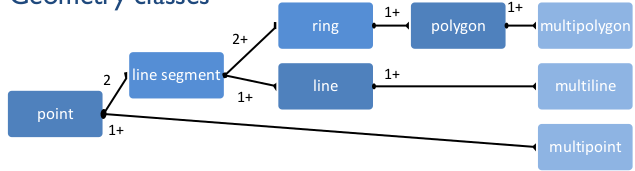
Multiple elements as one geometry
Geometry classes
Particularly suited to represent discrete objects
Relatively little memory requirements
Potentially infinite amount of precision
Discretization

Loss of information
Point • Pixel whose center is closest to the original point
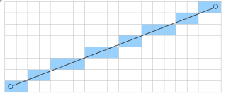
Line • Pixels intersecting the original line • Bresenham algorithm (1962)
Polygon
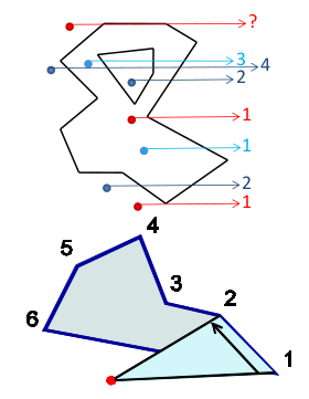
Point-in-polygon
Semi-line algorithm
Winding number algorithm
Polygon based fill algorithm
For each grid row

Ambiguous, manually control necessary
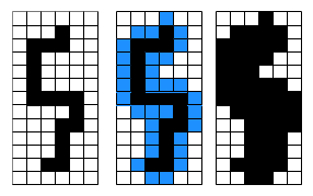
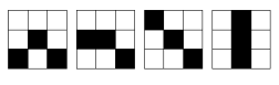
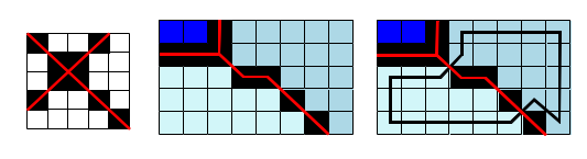
Input: binary image
Outline extraction for polygons
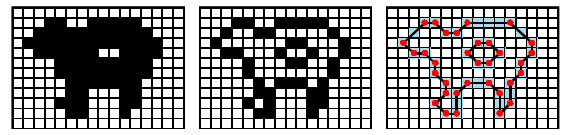
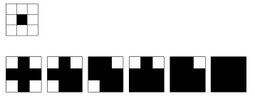
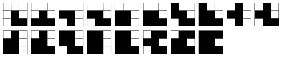
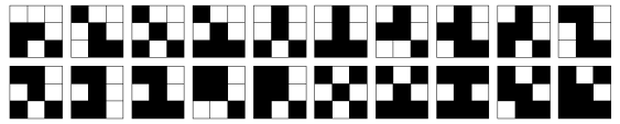
Topological thinning
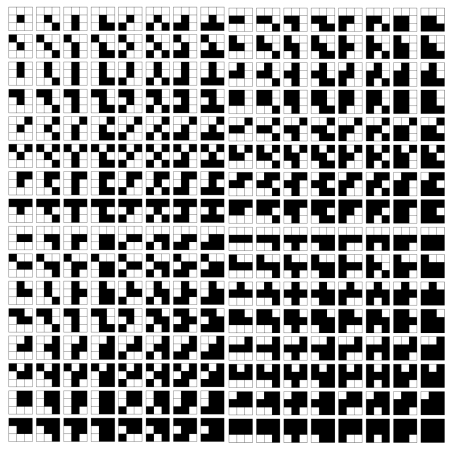
Classification of basic patterns results in 6 classes
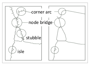
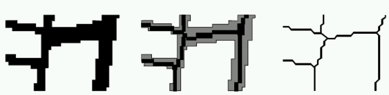
Centerline extraction for lines
Deficiencies
Raster topology
Metric space implies topological space, i.e. it is possible to determine the topological relations between objects if their geometries are known
Access and computations are normally more efficient if the topology is given explicitly
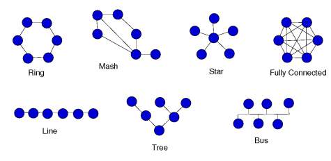
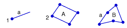
Basic elements of topological data models:
Relations
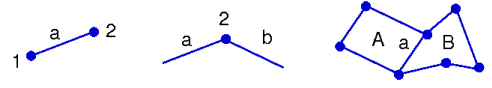
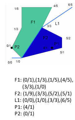
Spaghetti data structure
http://www.ikg.uni-hannover.de/lehre/katalog/gis/gisII_uebung
Spaghetti data structure
http://www.ikg.uni-hannover.de/lehre/katalog/gis/gisII_uebung
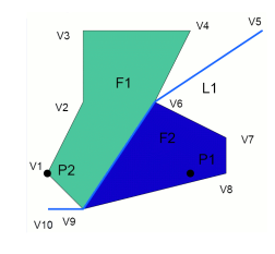
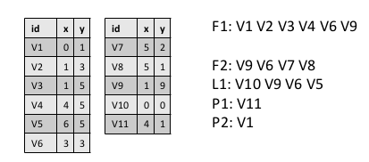
Edge list
http://www.ikg.uni-hannover.de/lehre/katalog/gis/gisII_uebung
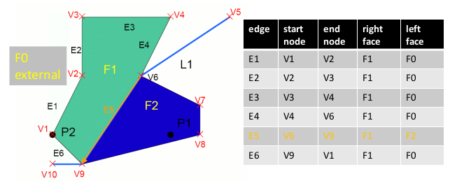
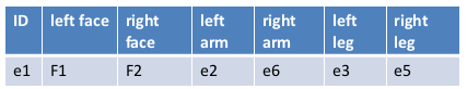
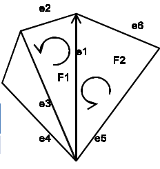
Winged edge (doubly connected edge list)
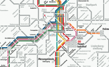
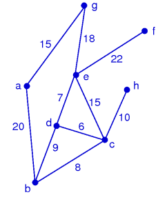
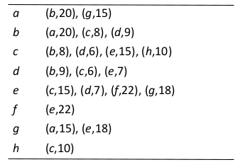
Network represented as weighted graph
{(ab,20), (ag,15), (bc,8), (bd,9), (cd,6), (ce,15), (ch,10), (de,7), (ef,22), (eg,18)}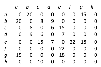
Adjacency list
Field-based models
Primary models
Derivative models
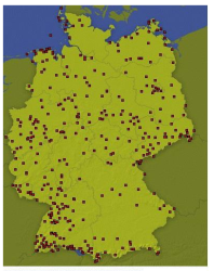
www.daserste.de/wetter/wetterstationen.asp
Display formats
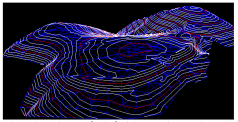
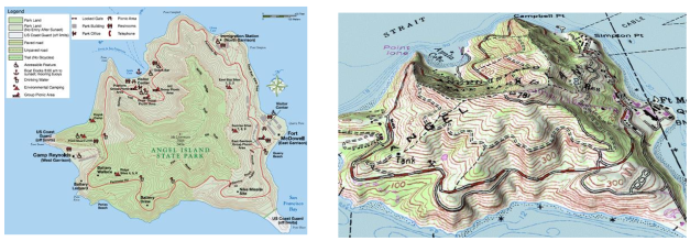
Isoline
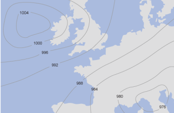
http://www.bbc.co.uk
Interpolation
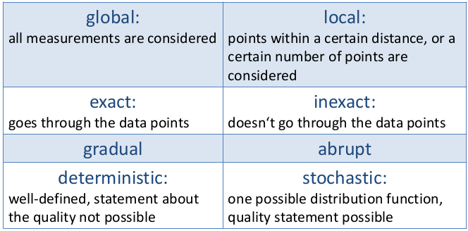
Nearest neighbour
http://skagit.meas.ncsu.edu/~helena/gmslab/interp/F1a.gif
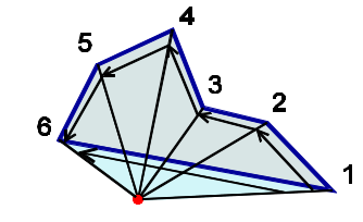
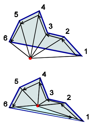
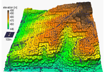
Surface constructed of triangular faces
Properties
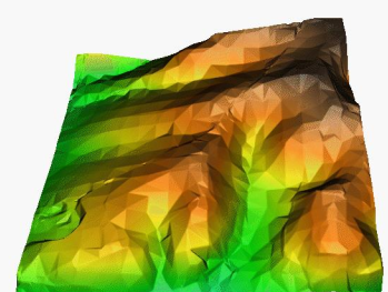
http://skagit.meas.ncsu.edu/~helena/gmslab/interp/F1b.gif
Discuss voronoi diagram?. 1page
Queries about this Session, please send them to:
*References*
- Geographic Information System Basics, 2012
J.E.Campbell & M. Shin- Fundamentals of GIS, 2017
Girmay Kindaya- GIS Applications for Water, Wastewater, and Stormwater Systems, 2005
U.M. Shamsi- Analytical and Computer Cartography, 2nd ed.
Keith C. Claike- Geographic Information Systems: The Microcomputer and Modern Cartography, 1st ed.
Fraser Taylor
Courtesy of Open School